Logistic Models in Machine Learning: A Beginner's Guide
May 5, 2025
This post provides a detailed overview of important logistic models in machine learning
Introduction
Prior to this post, I wrote about Linear Regression. You can check it out here.
Linear regression is fantastic for predicting continuous numerical values, like the price of a house, someone's height, or the temperature of tomorrow.
But what if you wanted to predict whether an email is spam or not spam? We are no longer predicting a number, we are predicting a category. Often times these are binary (two options) categories: spam or not spam.
Sigmoid Function
The Sigmoid Function lies at the heart of Logistic Regression. Let's say we have a function that takes any number as input and squishes it between 0 and 1.
- If you feed it a very large positive number, the output gets very close to 1.
- If you feed it a very large negative number, the output gets very close to 0.
- If you feed it 0, the output is exactly 0.5.
Visually, this represents an S-curve. The output of logistic regression always falls between 0 and 1, corresponding to "spam" or "no spam." If the sigmoid function outputs a value close to 1, the model predicts with high probability that the email is spam. If the output is close to 0, the model predicts with low probability that the email is spam (or high probability that it is not spam). If the output is around 0.5, the model is uncertain, assigning equal probability to the email being spam or not.
The Threshold
How can we get a definite classification of the email being spam or not spam? This is where we can use decision threshold. We choose a value between 0 and 1 to be our threshold (e.g. 0.5). This value can always be adjusted.
- If the predicted probability is greater than our treshold, we classify it as the positive class "spam"
- If the predicted probability is less than our treshold, we classify it as the negative class "not spam"
Imagine a doctor gets a test result for a patient indicating the probability of a certain condition is 0.7. The doctor needs to decide whether to start treatment or not. They might have a threshold: if the probability is above, say, 0.6 (the threshold), they recommend treatment. If it's below 0.6, they might recommend further monitoring instead. The threshold determines the action based on the probability.
Exercise
Let's say we have a logistic regression model for spam detection.
Spam Detection
| Probability | |
|---|---|
| A | 0.92 |
| B | 0.45 |
| C | 0.60 |
Q: Using a standard decision treshold of 0.5, how would you classify each email?
Email A (Prob = 0.92): Since 0.92 is greater than or equal to 0.5, it's classified as Spam.
Email B (Prob = 0.45): Since 0.45 is less than 0.5, it's classified as Not Spam.
Email C (Prob = 0.60): Since 0.60 is greater than or equal to 0.5, it's classified as Spam.
Log Loss
In Linear Regression we used a cost function like Mean Squared Error (MSE) to measure how far off the predictions were from the actual values.
Logistic Regression uses a different cost fuction called Log Loss, also called Binary Cross-Entropy. Log Loss is specifically for evaluating probabilistic predictions for binary classification.
- If the actual label is 1: The cost increases as the predicted probability gets closer to 0.
- If the actual label is 0: The cost increases as the predicted probability gets closer to 1.
The key benefits of using Log Loss are:
- Convexity: Log Loss creates a convex error langscape (like a bowl), making it much easier for optimization algorithms to find the best weights
- Penalty for Confident Errors. It heavily penalizes predictions that are confidently wrong, making the model more accurate
Let's look at a simple scenario where the actual class is 1 (spam).
- Scenario A: Model predicts probability = 0.6
- Scenario B: Model predicts probability = 0.1
Which scenario do you think Log Loss penalizes more heavily?
In this case 0.1 gets penalized more heavily because it's not just wrong, it's confidently wrong. The model is basicly saying "I'm pretty sure that this is not spam", when in fact, it is spam. Log Loss assigns a very high cost to such mistakes. The penalizing of confident errors is crucial for training effective classification models.
Logistic Algorithms
In this section we will go through some fundamental classification algorithms.
K-Nearest Neighbors (KNN)
How does it work:
- Choose 'k': You decide how many neighbors (k) to consider (e.g., k=3, k=5)
- Calculate Distances: When you get a new data point, calculate the distance from this new point to every single point in your training dataset
- Find Neighbors: Identify the 'k' training data points that have the smallest distances to the new point
- Majority Vote: Look at the class labels of these 'k' neighbors. The new data point is assigned the class that is most common among those 'k' neighbors
Suppose we are using a KNN for spam detection (Spam = 1, Not Spam = 0). We just received a new email we have to classify. We decided to use k=5. This means we calculated to distances and found the 5 closest emails in our training set with the following labels:
- Neighbor 1: Spam (1)
- Neighbor 2: Not Spam (0)
- Neighbor 3: Spam (1)
- Neighbor 4: Spam (1)
- Neighbor 5: Not Spam (0)
Based on this, how would our KNN model classify the new model?
3 out of 5 nearest neighbors are Spam and only 2 are Not Spam. Therefore, the KNN algorithm predicts that the new email is SPAM!
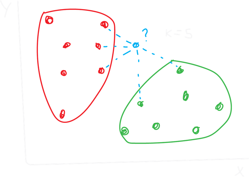
Logistic Regression KNN Example
Support Vector Machines (SVM)
SVM is another powerful classification algorithm. It also has some similarities with Support Vector Regression (SVR) explained in my other post. The core idea is to find the optimal hyperplane (which is just a boundary line) that best seperates the different classes. With this, SVM tries to maximize the margin.
- Think of margin as a street. The edges of the street touch the closest data points from each class. SVM tries to make this street as wide as possible.
- The data points that lie exactly on the edges of this margin are called the support vectors. If you were to move these points, the optimal hyperplane might change. Points further away don't influence the boundary directly.
Imagine a river separating two villages, red and blue. You want to build a fence between them so villagers don’t cross into the wrong area. Instead of building it right next to one village, you place it exactly in the middle of the widest part of the river, the place that’s equally far from both.
That’s the SVM idea:
Build a boundary that maximizes the margin between the closest red and blue points.
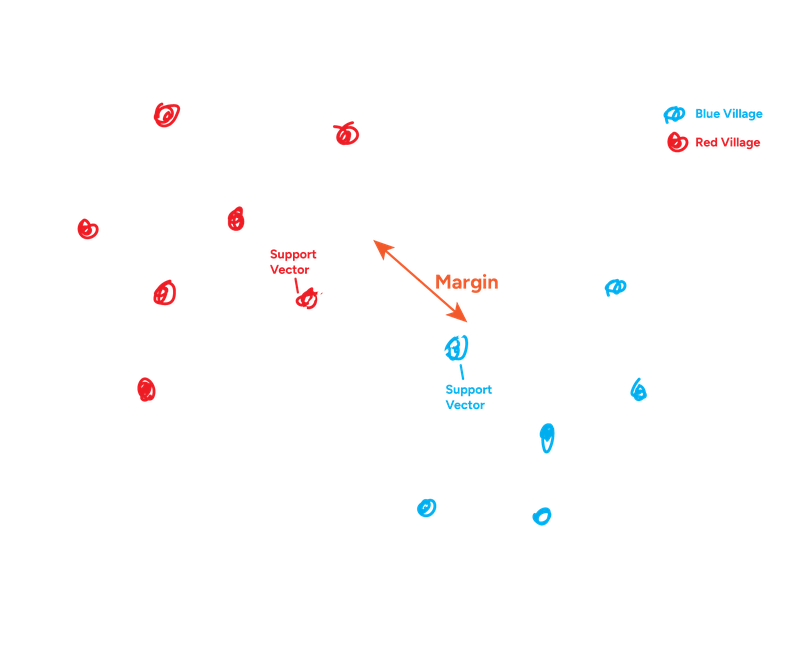
Support Vector Machine - Example
So, the core idea of the basic (linear) SVM is finding the maximum margin hyperplane, defined by the support vectors.
This explanation covers the case where the data is linearly separable, meaning you can draw a straight line to perfectly separate the classes.
What do you think happens if the data isn't linearly separable? Can you draw a single straight line to separate them? This leads us to the next into the concept of SVM Kernels, which we will discuss next.
SVM Kernels
So what if the data points are mixed up in a way that no single straight line can neatly separate them? Think of a cluster of blue dots surrounded by a ring of red dots. This is where we can use the SVM Kernel Trick.
The core idea is to project the data into a higher-dimensional space where it does become linearly separable. Then, SVM finds the maximum margin hyperplane in that higher dimension.
Radial Basis Function (RBF) is one of the most popular and powerful kernels. It maps data into an infinite-dimensional space! Think of it as creating "bumps" around data points.
Lets say we have red and blue dots scattered on a piece of paper (2D) such that we can't draw a single straight line to separate them. What if we could somehow lift the blue dots up off the paper into a third dimension (making it 3D). Now you can place a flat sheet of paper between the lifted blue dots and the red dots still on the original paper.
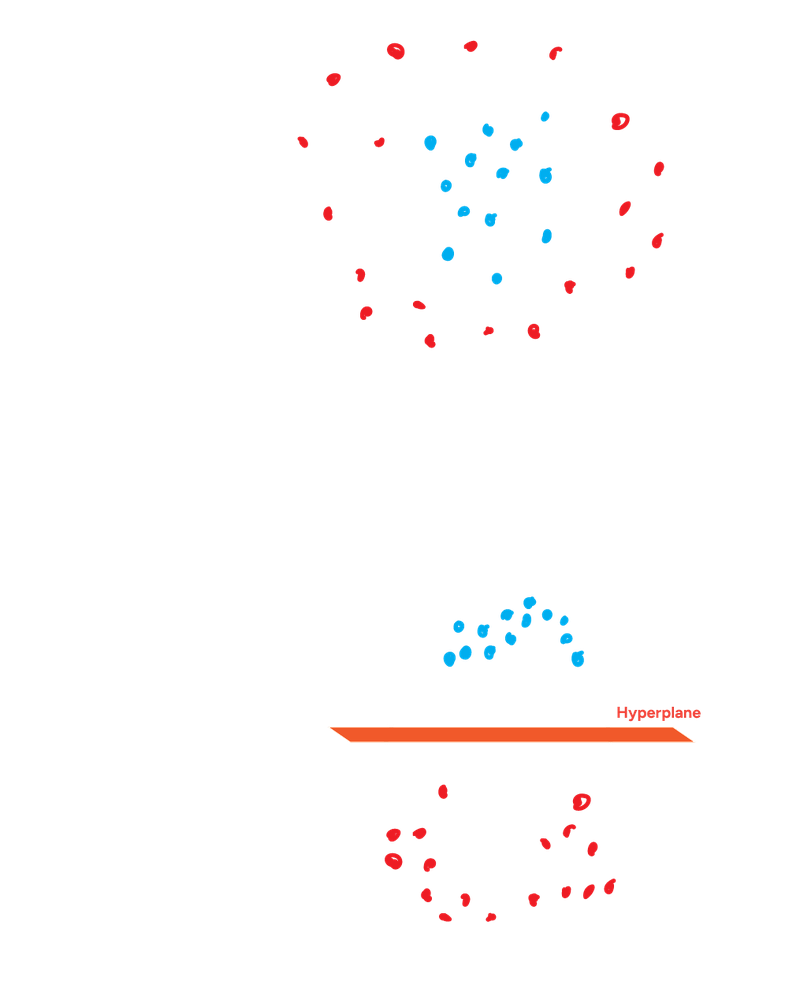
SVM Kernel Trick - Example
SVM & Kernels:
- SVM: Find the hyperplane with the maximum margin between classes.
- Kernel Trick: Handles non-linearly separable data by mapping to higher dimensions using kernel functions (like RBF).
Decision Tree
A decision tree is like a flowchart used for both classification and regression. For classification, it works by splitting the data based on the values of its features, creating a tree where:
- Internal Nodes: Represent a test on a feature (Is email word count > 500?)
- Branches: Represent the outcome of the test (Yes or No)
- Leaf Nodes: Represent the final classification (Spam or Not Spam)
You start at the top (the root node) and traverse down the tree by answering the questions at each node until you reach a leaf node, which gives you the predicted outcome.
Below a simple tree for predicting if someone will play tennis:
-  Today's Outlook?
       /   |   \
   Sunny  Overcast  Rainy
    /       |       \
Humidity?   YES     Windy?
 /     \           /    \
High   Normal     True  False
 |       |        |      |
 NO     YES       NO     YES
Using the simple tennis decision tree, predict whether someone will play tennis given the following conditions:
- Outlook: Sunny
- Humidity: High
As also discussed in my other post on linear regression models, we face the same overfitting problem here. If you have a huge dataset with lots of features, and you include all of them, the model might just memorize the training data, but perform badly on new, unseen data.
This leads us to the next algorithm on the list, which was designed specifically to combat this problem.
Random Forest
A Random Forest is an ensemble learning (multiple models) method. Instead of relying on a single Decision Tree, it builds many decision trees during training and combines their outputs to make a final prediction. The core idea is that by averaging the predictions of many diverse trees, the final model becomes more robust and accurate, overcoming the main weakness of individual decision trees (overfitting).
So how does it exactly prevent overfitting?
Each tree is build with a subset of the data. This means that each tree will learn slightly different patterns. This is also called Bagging.
The second thing is that each tree will also only have a restricted amount of features to choose from. This way they will have to explore different ways to partition the data. So, the combination of data randomness and feature randomness creates a diverse bunch of trees, and the final decision is much more generalizable (ability to perform well on unseen data) than any single tree's decision.
You need to make an important decision (diagnosing a patient). Instead of relying on just one doctor (one decision tree), you consult a large committee of doctors (the forest).
fin.
Test your knowledge
1. What type of problem is Logistic Regression primarily used for, and what kind of output does it produce?
It's used for binary classification problems (predicting one of two categories). It outputs a probability (between 0 and 1)
2. What is the name and shape of the function used in Logistic Regression to convert a linear combination of inputs into a probability?
Sigmoid
3. What cost function is typically used to train a Logistic Regression model?
Log Loss
4. How does the K-Nearest Neighbors (KNN) algorithm classify a new data point?
It finds the 'k' data points in the training set that are closest to the new point and assigns the class that is the majority among those 'k' neighbors
5. Why is feature scaling (normalization or standardization) often crucial before applying KNN?
Because KNN relies on distance calculations. Features with larger ranges can dominate the distance metric if not scaled, leading to biased results
6. What is the main goal of a linear Support Vector Machine (SVM) when finding a decision boundary?
To find the hyperplane that has the maximum margin
7. What are the "support vectors" in an SVM?
They are the data points from the training set that lie exactly on the edges of the margin
8. What is the purpose of using Kernels (like RBF or Polynomial) with SVMs?
Kernels allow SVMs to effectively classify data that is not linearly separable by mapping the data to a higher-dimensional space
9. How does a Decision Tree make a prediction for a new data point?
The data point traverses down the tree from the root node, following the branches based on the outcomes of tests on its feature values at each internal node, until it reaches a leaf node which contains the final prediction
10. What is the primary disadvantage of a single, deep Decision Tree?
Overfitting
11. What type of algorithm is a Random Forest, and what does it combine?
It's an ensemble (multiple models) algorithm that combines multiple Decision Trees
12. What are the two main sources of randomness introduced when building a Random Forest to ensure diversity among the trees?
Training each tree on a random subset of the data. Considering only a random subset of features at each split point in each tree.
13. How does a Random Forest make a final classification prediction?
Each tree in the forest makes an individual prediction, and the Random Forest outputs the class that receives the majority of the votes.